import graphviz

# This output is generated from the model
# as you can see, there are several decisions
# to make, and the hyrarchy can be compiled like a tree
graphviz.Source.from_file('cache/iristree.dot')
import graphviz
# This output is generated from the model
# as you can see, there are several decisions
# to make, and the hyrarchy can be compiled like a tree
graphviz.Source.from_file('cache/iristree.dot')
first we need to import pandas and load the data with pd.read_csv(file)
import pandas as pd

iris = pd.read_csv('datasets/iris/Iris.csv')
this is the overview of the data
iris| Id | SepalLengthCm | SepalWidthCm | PetalLengthCm | PetalWidthCm | Species | |
|---|---|---|---|---|---|---|
| 0 | 1 | 5.1 | 3.5 | 1.4 | 0.2 | Iris-setosa |
| 1 | 2 | 4.9 | 3.0 | 1.4 | 0.2 | Iris-setosa |
| 2 | 3 | 4.7 | 3.2 | 1.3 | 0.2 | Iris-setosa |
| 3 | 4 | 4.6 | 3.1 | 1.5 | 0.2 | Iris-setosa |
| 4 | 5 | 5.0 | 3.6 | 1.4 | 0.2 | Iris-setosa |
| ... | ... | ... | ... | ... | ... | ... |
| 145 | 146 | 6.7 | 3.0 | 5.2 | 2.3 | Iris-virginica |
| 146 | 147 | 6.3 | 2.5 | 5.0 | 1.9 | Iris-virginica |
| 147 | 148 | 6.5 | 3.0 | 5.2 | 2.0 | Iris-virginica |
| 148 | 149 | 6.2 | 3.4 | 5.4 | 2.3 | Iris-virginica |
| 149 | 150 | 5.9 | 3.0 | 5.1 | 1.8 | Iris-virginica |
150 rows × 6 columns
if we wan to check detail about the data, use data.info()
iris.info()<class 'pandas.core.frame.DataFrame'>
RangeIndex: 150 entries, 0 to 149
Data columns (total 6 columns):
# Column Non-Null Count Dtype
--- ------ -------------- -----
0 Id 150 non-null int64
1 SepalLengthCm 150 non-null float64
2 SepalWidthCm 150 non-null float64
3 PetalLengthCm 150 non-null float64
4 PetalWidthCm 150 non-null float64
5 Species 150 non-null object
dtypes: float64(4), int64(1), object(1)
memory usage: 7.2+ KBthe Id is not needed in this case, therefore we can just drop it
# stropping unneeded data
iris.drop('Id', axis=1, inplace=True)| Id | SepalLengthCm | SepalWidthCm | PetalLengthCm | PetalWidthCm | Species | |
|---|---|---|---|---|---|---|
| 0 | 1 | 5.1 | 3.5 | 1.4 | 0.2 | Iris-setosa |
| 1 | 2 | 4.9 | 3.0 | 1.4 | 0.2 | Iris-setosa |
| 2 | 3 | 4.7 | 3.2 | 1.3 | 0.2 | Iris-setosa |
| 3 | 4 | 4.6 | 3.1 | 1.5 | 0.2 | Iris-setosa |
| 4 | 5 | 5.0 | 3.6 | 1.4 | 0.2 | Iris-setosa |
now, we separate the data label from its features, and save it to X and y, we need also to separate the data to train and split
X = iris[['SepalLengthCm', 'SepalWidthCm', 'PetalLengthCm', 'PetalWidthCm']]
y = iris['Species']

from sklearn.model_selection import train_test_split
X_train, X_test, y_train, y_test = train_test_split(X, y, test_size=0.1, random_state=123)
we prepare the model by calling it from sklearn.tree
from sklearn import tree

clf = tree.DecisionTreeClassifier()
# With defined train test split
clf = clf.fit(X_train, y_train)cross_val_score is for validating the quality of data set, it’s consider good if it’s more than 0.85
# with cross validation
from sklearn.model_selection import cross_val_score

scores = cross_val_score(clf, X, y, cv=5)scoresarray([0.96666667, 0.96666667, 0.9 , 0.96666667, 1. ])# model evaluation
from sklearn.metrics import accuracy_score
y_pred = clf.predict(X_test)
print(y_pred)
print(y_test)
acc_score = round(accuracy_score(y_pred, y_test), 3)
print('accuracy', acc_score)['Iris-virginica' 'Iris-virginica' 'Iris-virginica' 'Iris-versicolor'
'Iris-setosa' 'Iris-virginica' 'Iris-versicolor' 'Iris-setosa'
'Iris-setosa' 'Iris-versicolor' 'Iris-virginica' 'Iris-setosa'
'Iris-versicolor' 'Iris-virginica' 'Iris-virginica']
72 Iris-versicolor
112 Iris-virginica
132 Iris-virginica
88 Iris-versicolor
37 Iris-setosa
138 Iris-virginica
87 Iris-versicolor
42 Iris-setosa
8 Iris-setosa
90 Iris-versicolor
141 Iris-virginica
33 Iris-setosa
59 Iris-versicolor
116 Iris-virginica
135 Iris-virginica
Name: Species, dtype: object
accuracy 0.933print(clf.predict([[6.2, 3.4, 5.4, 2.3]])[0])from sklearn.tree import export_graphviz
export_graphviz(
clf,
out_file = 'cache/iristree.dot',
feature_names = ['SepalLengthCm', 'SepalWidthCm', 'PetalLengthCm', 'PetalWidthCm'],
class_names = ['Iris-setosa', 'Iris-versicolor', 'Iris-virginica' ],
rounded= True,
filled =True)import numpy as np
# make dummy data of rooms
bedrooms = np.array([1,1,2,2,3,4,4,5,5,5])
# make dummy price data in dolar
house_price = np.array([15000, 18000, 27000, 34000, 50000, 68000, 65000, 81000,85000, 90000])# visualize in scatterplot
import matplotlib.pyplot as plt
%matplotlib inline
plt.scatter(bedrooms, house_price)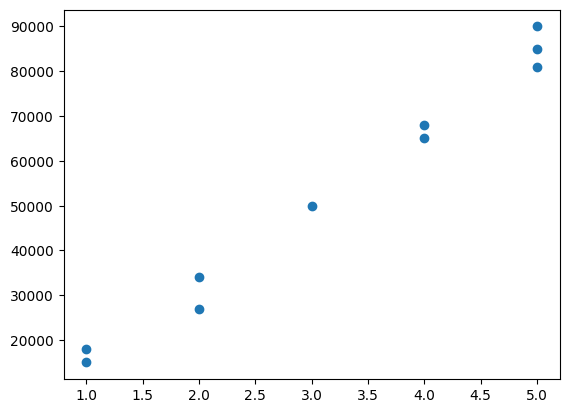
from sklearn.linear_model import LinearRegression

# train the model with LinearRegression.fit()
bedrooms = bedrooms.reshape(-1, 1)
linreg = LinearRegression()
linreg.fit(bedrooms, house_price)LinearRegression()In a Jupyter environment, please rerun this cell to show the HTML representation or trust the notebook.
LinearRegression()
# plotting the corelation between number of rooms and house_prices
plt.scatter(bedrooms, house_price)
plt.plot(bedrooms, linreg.predict(bedrooms))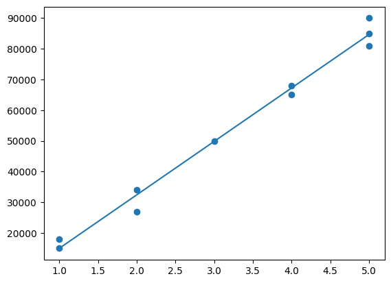
import pandas as pd

df = pd.read_csv('datasets/socmedAds/Social_Network_Ads.csv')
df| User ID | Gender | Age | EstimatedSalary | Purchased | |
|---|---|---|---|---|---|
| 0 | 15624510 | Male | 19 | 19000 | 0 |
| 1 | 15810944 | Male | 35 | 20000 | 0 |
| 2 | 15668575 | Female | 26 | 43000 | 0 |
| 3 | 15603246 | Female | 27 | 57000 | 0 |
| 4 | 15804002 | Male | 19 | 76000 | 0 |
| ... | ... | ... | ... | ... | ... |
| 395 | 15691863 | Female | 46 | 41000 | 1 |
| 396 | 15706071 | Male | 51 | 23000 | 1 |
| 397 | 15654296 | Female | 50 | 20000 | 1 |
| 398 | 15755018 | Male | 36 | 33000 | 0 |
| 399 | 15594041 | Female | 49 | 36000 | 1 |
400 rows × 5 columns
df.info()<class 'pandas.core.frame.DataFrame'>
RangeIndex: 400 entries, 0 to 399
Data columns (total 5 columns):
# Column Non-Null Count Dtype
--- ------ -------------- -----
0 User ID 400 non-null int64
1 Gender 400 non-null object
2 Age 400 non-null int64
3 EstimatedSalary 400 non-null int64
4 Purchased 400 non-null int64
dtypes: int64(4), object(1)
memory usage: 15.8+ KBdata = df.drop(columns=['User ID'])
data = pd.get_dummies(data)
data| Age | EstimatedSalary | Purchased | Gender_Female | Gender_Male | |
|---|---|---|---|---|---|
| 0 | 19 | 19000 | 0 | False | True |
| 1 | 35 | 20000 | 0 | False | True |
| 2 | 26 | 43000 | 0 | True | False |
| 3 | 27 | 57000 | 0 | True | False |
| 4 | 19 | 76000 | 0 | False | True |
| ... | ... | ... | ... | ... | ... |
| 395 | 46 | 41000 | 1 | True | False |
| 396 | 51 | 23000 | 1 | False | True |
| 397 | 50 | 20000 | 1 | True | False |
| 398 | 36 | 33000 | 0 | False | True |
| 399 | 49 | 36000 | 1 | True | False |
400 rows × 5 columns
X = data[['Age', 'EstimatedSalary', 'Gender_Female', 'Gender_Male']]
y = data['Purchased']
# data normalization
from sklearn.preprocessing import StandardScaler
scaler = StandardScaler()
# calculating the mean and standard deviation of every attribute column
# to be used on every transform function
scaler.fit(X)
scaled_data = scaler.transform(X)
scaled_data = pd.DataFrame(scaled_data, columns=X.columns)
scaled_data| Age | EstimatedSalary | Gender_Female | Gender_Male | |
|---|---|---|---|---|
| 0 | -1.781797 | -1.490046 | -1.020204 | 1.020204 |
| 1 | -0.253587 | -1.460681 | -1.020204 | 1.020204 |
| 2 | -1.113206 | -0.785290 | 0.980196 | -0.980196 |
| 3 | -1.017692 | -0.374182 | 0.980196 | -0.980196 |
| 4 | -1.781797 | 0.183751 | -1.020204 | 1.020204 |
| ... | ... | ... | ... | ... |
| 395 | 0.797057 | -0.844019 | 0.980196 | -0.980196 |
| 396 | 1.274623 | -1.372587 | -1.020204 | 1.020204 |
| 397 | 1.179110 | -1.460681 | 0.980196 | -0.980196 |
| 398 | -0.158074 | -1.078938 | -1.020204 | 1.020204 |
| 399 | 1.083596 | -0.990844 | 0.980196 | -0.980196 |
400 rows × 4 columns
# validation with cross validation
from sklearn.model_selection import cross_val_score
from sklearn import linear_model

model = linear_model.LogisticRegression()
scores = cross_val_score(model, scaled_data, y, cv=5)scoresarray([0.7 , 0.95 , 0.9375, 0.8125, 0.7 ])from sklearn.model_selection import train_test_split
X_train, X_test, y_train, y_test = train_test_split(scaled_data, y, test_size=0.2, random_state=1)model.fit(X_train, y_train)LogisticRegression()In a Jupyter environment, please rerun this cell to show the HTML representation or trust the notebook.
LogisticRegression()
# examine model accuracy
model.score(X_test, y_test)
0.825